Camera Modeling, Part 4: Pinhole Obsession
Pinhole Obsession is a dangerous condition that can occur after years spent in proximity to computer vision labs, researchers, and startups.
Devon Morris
Staff Perception Engineer
Oct 15, 2024

Explore our entire Camera Modeling Series:
Part I: Focal Length And Collinearity
Part 2: Introducing Lens Distortion
Part 3: Exploring Distortion and Distortion Models
Part 4: Pinhole Obsession
Part 5: The Deceptively Asymmetric Unit Sphere
If you’d like to be notified of when that next post drops, just follow us on LinkedIn or subscribe to our newsletter.
—
In a previous post on distortion models, we explored the difference between forward and inverse distortion models, their uses and the geometry they describe. However, up to this point in all three of our blog posts on camera modeling, we’ve fallen into the trap of Pinhole Obsession.
Pinhole Obsession
If you’ve ever heard the phrase “assume a pinhole camera,” and simply nodded your head in agreement, you may be guilty of Pinhole Obsession. If you’ve ever said “I can’t handle these points, because they are behind the camera,” you may be guilty of Pinhole Obsession. If you’ve ever divided by \(Z\) and assumed a positive depth, you may be guilty of Pinhole Obsession. If you’ve ever thought that rays, pixel coordinates and normalized image plane coordinates are basically the same thing, you may be guilty of Pinhole Obsession.
Pinhole Obsession is the careless method of modeling all cameras as a projection from the positive-depth half-space into pixel coordinates. Stated similarly, Pinhole Obsession is when a model creates a correspondence between real-world 3D object space points and normalized image plane coordinates by simply dividing by depth. This fascination with the pinhole camera model even applies to cameras with distortion, which are either modeled as some distortion in normalized image plane coordinates or an inverse distortion applied to centered image coordinates.
If you look in all the classic textbooks, and in many computer vision libraries this is typically how cameras are modeled, so you may be left asking “why the hate for the pinhole camera?” Simply stated, it is not the geometrically correct model. The standard-issue 20 oz. hammer in every computer vision engineer’s toolbox is the pinhole camera. When all we have is this hammer, we make every computer vision problem into a nail that we can hit. In this process, we leave behind a number of broken screws, a few 2x4s with dents in them and a still unfinished bathroom remodel (true story). Our fascination with the pinhole model hamstrings our ability to solve computer vision problems in the real-world, and these real-world problems start to appear when our camera’s field-of-view widens.
⚠️ OpenCV’s fisheye model, despite appearing to support wide field-of-view cameras, falls into the Pinhole Obsession trap by first creating a correspondence between object space points and normalized image plane coordinates by dividing by depth. As such, this model cannot handle very wide field-of-view cameras and does not understand anything about points “behind the camera.”
Wide Field of View Cameras
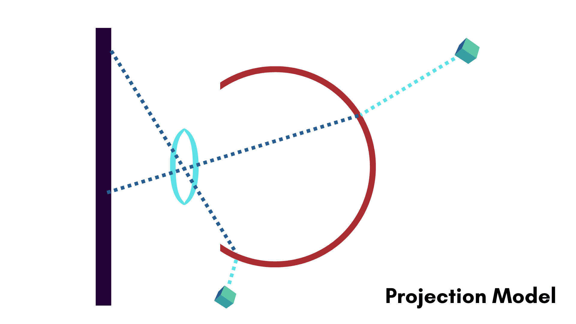
Once a camera begins to approach 120° diagonal field-of-view (DFOV), our traditional method of modeling cameras as a pinhole with distortion begins to break down. When discussing various FOVs, we at Tangram generally refer to such cameras with greater than 120° DFOV as wide field-of-view (WFOV) cameras. To illustrate how the pinhole model breaks down for WFOV cameras, imagine a pinhole camera that’s sitting at the center of a half-sphere that we want to image. Here is a cross section of this imaging system.
Click on image to view a larger version
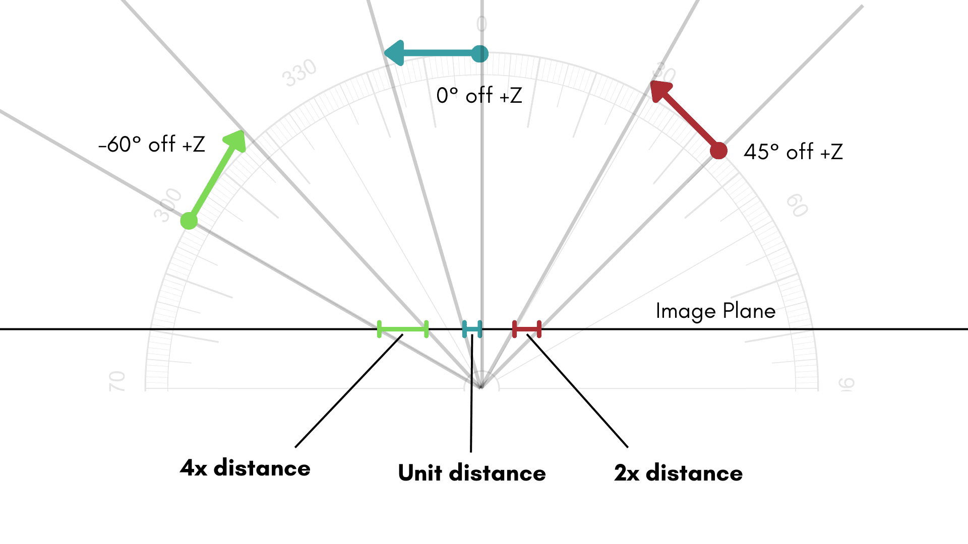
Now imagine a point moving along this sphere. When the point is directly in front of the camera, a change in one unit along the sphere maps to a change in one unit along the normalized image plane. When the point is 30° a change in one unit along the sphere maps to a change in 1.33 units along the normalized image plane. Consider the following table of induced distances on the normalized image plane.
Degrees from +Z | Induced Distance On The Normalized Image Plane |
|---|---|
0° | 1.00 |
30° | 1.33 |
45° | 2.00 |
60° | 4.00 |
75° | 14.93 |
80° | 33.16 |
85° | 131.60 |
90° | ∞ |
Admittedly, these are idealized numbers and a camera with a finitely-sized imager will eventually have these points fail to project on the imaging surface. But in the very realistic case where we are using a 120° DFOV camera, there is a dilation of real-world misalignments by at least a factor of four on the edges of the image!
As the camera’s field-of-view approaches 180° DFOV, this model completely breaks and fails to express any change caused by movement of the 3D point. If a camera has more than a 180° DFOV it becomes unclear how to handle any points behind the camera with the pinhole model alone; In contrast, there exist examples of camera systems that can image points that are physically behind the camera. A common misconception held by computer vision engineers is to think that points behind the camera are off limits in some regard. Behind the camera does not imply outside of the field-of-view as the following photo demonstrates.
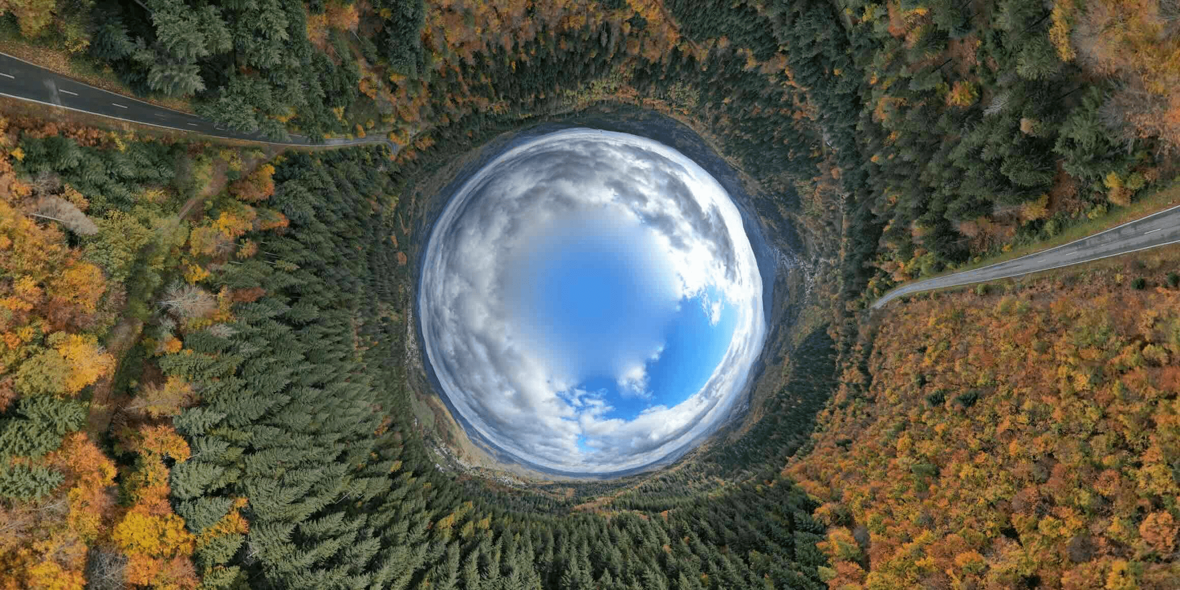
Image credit: Photo by Bernd 📷 Dittrich on Unsplash
A geometrically correct camera model should be able to describe the correspondence between any pixel on the image and the ray of light in the real-world that landed in that pixel well. The only points that are off limits are ones that do not cast light onto the camera’s imaging surface.
These are the problems with Pinhole Obsession: non-uniform weighting of 3D information on the normalized image plane and the inability to describe the 3D structure of all pixels in an image. So, how do we solve these problems?
Rays vs. Camera Rays
To solve the problems associated with Pinhole Obsession, we first have to understand why it exists. Some reasons include:
Pedagogy of pinhole camera is much simpler than alternatives
Common computer vision libraries focus exclusively on pinhole cameras
Pinhole cameras and associated distortion models are “good enough” in most cases, especially if you are using standard field-of-view cameras
Despite this, we as a community of computer vision engineers have been far too cavalier with the word ray. A camera is essentially a device that converts rays of light into pixel coordinates, “projecting” out the distance information in the process. The layman would define a ray as “a line emanating from an object.” As computer vision engineers, we may interpret this as the line from an object to the perspective center of a camera. However, this simplistic line of thinking leads to the aforementioned Pinhole Obsession. Consequently, we must define in very real and mathematical terms what a ray is. It turns out that there are two conflicting ways to think about rays: rays in the real-world and rays that necessarily interact with the camera’s imaging surface.
Camera Rays
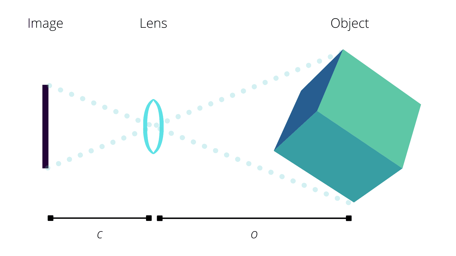
First, consider the imaging surface of the camera. You may imagine the perspective center of this camera as a point which sits in front of the CMOS through which beams of light travel. This imaging surface has finite dimensions and is generally assumed to be flat; as such, it is reasonable to assume that the entire imaging surface lies behind the perspective center of the camera. Since the imaging surface lies behind the perspective center of the camera, only beams of light that are in front of the perspective center will intersect the imaging surface on its photoreceptive side.
💡 Computer vision engineers and photogrammetrists differ on whether to view the imaging surface as in front of or behind the perspective center of the camera. The two conventions are geometrically equivalent and only differ in representation by a change of sign. The distinguishing property of this model is that imaged points are restricted to a half space of \(\mathbb{R}^3\), which is true regardless of convention.
Since all beams of light that are imaged lie in front of the perspective center of the camera, we can safely assume that the object’s \(Z\) is positive and can write the homogeneous coordinates as
$$\begin{bmatrix}x \\y \\1\end{bmatrix}=\begin{bmatrix}X / Z \\Y / Z \\1\end{bmatrix}$$
But what are homogeneous coordinates anyway? They are the canonical element of an equivalence class where the equivalence relation is given by
$$\begin{bmatrix}x_1 \\y_1 \\z_1\end{bmatrix} \sim \lambda \begin{bmatrix}x_2 \\y_2 \\z_2\end{bmatrix}, \lambda \in \mathbb{R}^{+}, z_1 > 0, z_2 > 0$$
If that’s too much math jargon, then just say that a camera ray is a directed line that must pass through the camera’s imaging surface. This line must pass through the normalized image plane where \(Z = 1\), and we don’t regard points “behind the camera” as being on this line. Thus, the homogeneous coordinates of this camera ray is the point where the camera ray intersects with the normalized image plane. This is the traditional computer vision way of modeling rays, and it gives rise to the pinhole projection model.
💡 In precise mathematical terms, this set of rays is called the oriented real projective plane and is commonly denoted by \(\mathbb{T}^2\). If you’ve seen this terminology before, you’ll notice that this is a torus. This is because in real-projective geometry, we also add the points and lines “at infinity”.
These extra points can be regarded as the points where the left side of image “wraps around” to the right side of the image and the top of the image “wraps around” to the bottom side of the image. This wrapping behavior forms the same structure as a torus. However, it is rare to do computation with these extra points at infinity in practice, since a camera’s imaging surface is finitely sized.
Now you can brag to all your friends about your math knowledge and say weird things like “an ideal pinhole camera is a donut.”
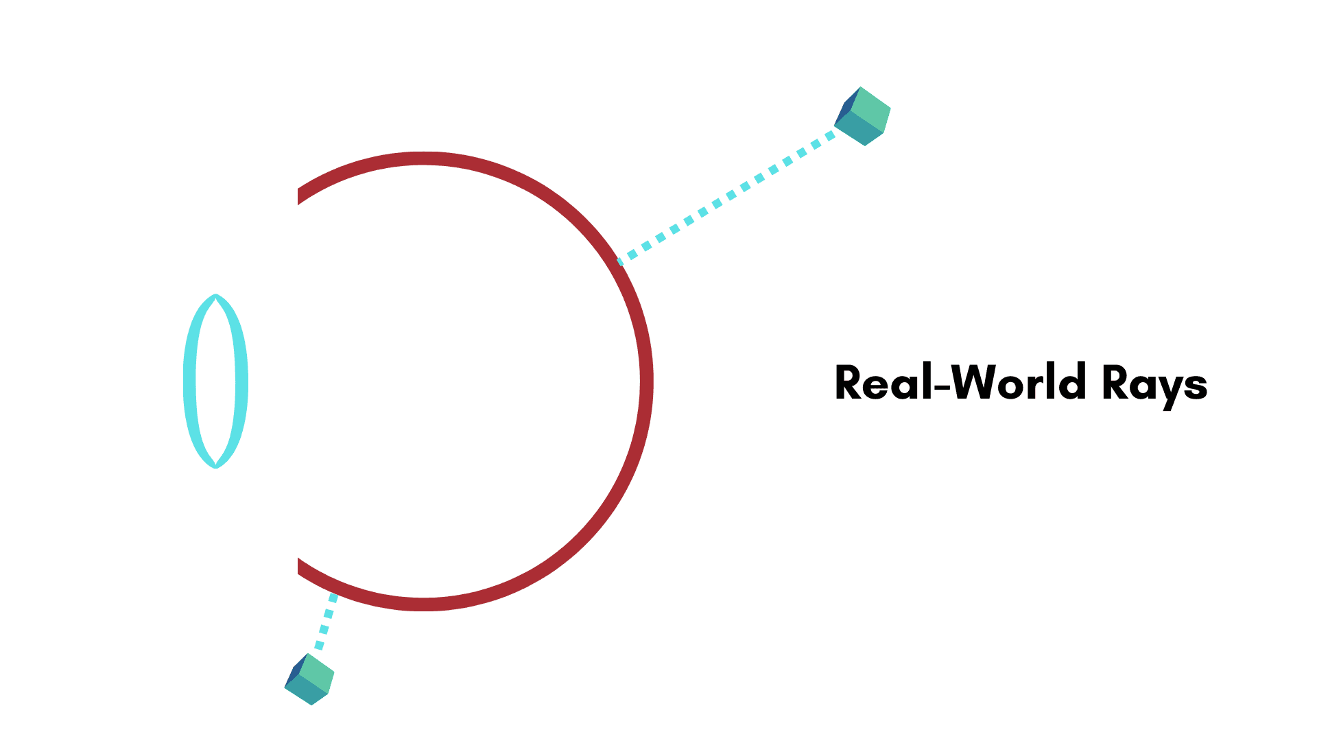
Real-World Rays
Now, consider the object space — points in 3D in the real-world. You may imagine a point anywhere in 3D space, and a line that connects this point to the perspective center of the camera. Note that the line that connects these two points can be in front of the imager, or it can be behind the imager. Really, we aren’t even thinking about the imaging surface at all when we think of rays like this.
Similar to camera rays, we can define these rays as an equivalence class.
$$
\begin{bmatrix}
x_1 \\
y_1 \\
z_1
\end{bmatrix} \sim \lambda
\begin{bmatrix}
x_2 \\
y_2 \\
z_2
\end{bmatrix}
, \lambda \in \mathbb{R}^{+}
$$
Essentially, there is only one difference from camera rays: the restriction on \(z_1\) and \(z_2\) is lifted. We still disallow the ray passing beyond the perspective center of the camera (\(\lambda\) as a negative number), since we regard that as a distinct ray coming from the opposite side of the camera. Again, it is necessary to choose some canonical member of this equivalence class, referred to as the “ray coordinates.” The ray coordinates for a point are given as:
$$
\begin{bmatrix}
x \\
y \\
z
\end{bmatrix} =
\frac{1}{\sqrt{X^2 + Y^2 + Z^2}}\begin{bmatrix}
X \\
Y \\
Z
\end{bmatrix}
$$
Seeing the canonical ray coordinates, it should become very obvious that the mathematical object we are dealing with here is the unit sphere \(\mathcal{S}^2\). However, now we are stuck with two different ways to think about rays. How do we bridge the gap?
Projection Models
The secret to unifying these two disparate views of rays is crafting a geometrically correct projection model. Simply put, our projection model should map points to rays, rays to camera rays and camera rays to pixels. Mathematically, we have
$$
\begin{aligned}
&\pi : \mathbb{R}^3 \to \mathcal{S}^2 \\
&\mu : \mathcal{S}^2 \to \mathbb{T}^2 \\
&\kappa : \mathbb{T}^2 \to \mathbb{R}^2 \\
&\kappa \circ \mu \circ \pi : \mathbb{R}^3 \to \mathbb{R}^2
\end{aligned}
$$
where \(\pi\) is the projection from points to rays, \(\mu\) is the modeling function that maps rays into camera rays and \(\kappa\) converts camera rays into pixels.
This is the big secret and the solution to Pinhole Obsession. Creating a projection model in this fashion even works for the inverse models in our previous blog post, we just have to numerically calculate \(\mu\) from \(\mu^{-1}\) if no closed-form modeling function exists.
💡 If you read about the wide field-of-view models we support and also read the corresponding papers through this lens of projection, it will become evident that all camera models just convert real-world rays to camera rays at some point in their projection model.
Real-world Rays on a Real Dataset, for Real
With a geometrically correct projection model it is possible to compose \(\mu^{-1} \circ \kappa^{-1}\), thus mapping pixels back to real-world rays. This formulation allows us to perform calculations and optimization with rays instead of pixel coordinates.
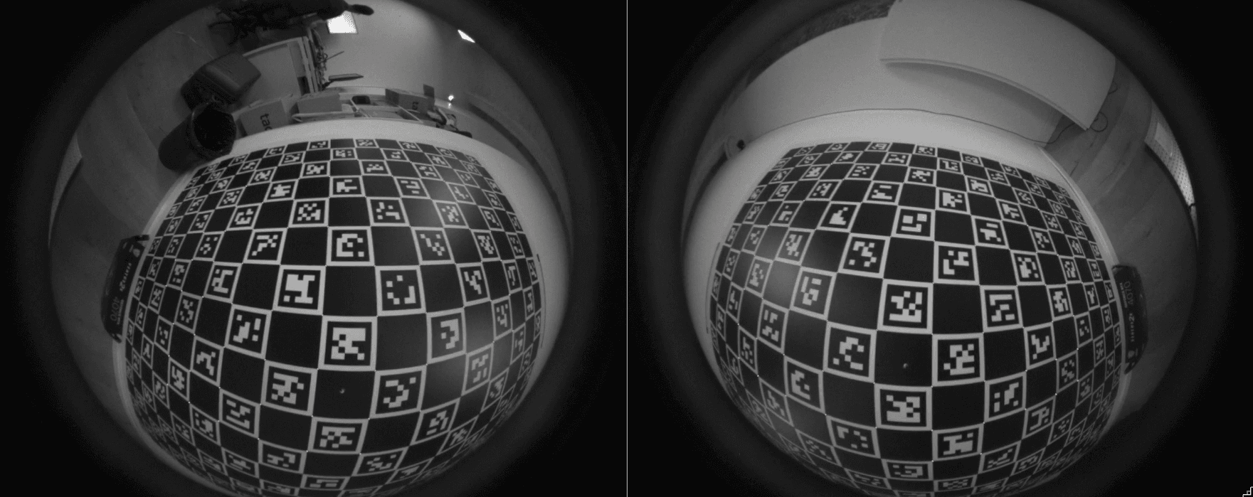
Consider the common use-case of camera calibration: given some data collected of a markerboard, we want to infer this projection model \(\kappa \circ \mu \circ \pi\) based on detected coordinates in the image. Here is a single frame from a calibration dataset with WFOV cameras.
Here’s what the reprojection error looks like when we minimize pixel misalignment for this calibration data. You can click on each image to view a larger version.

This calibration looks fairly good! However, there remains something lurking beneath the surface. Let’s take a different view of this same calibration, but consider the ray alignment error of these same points

As you can see, the ray alignment, which represents real-world 3D alignment, is slightly biased in favor of in the center of the image. Now let’s minimize over ray alignment.


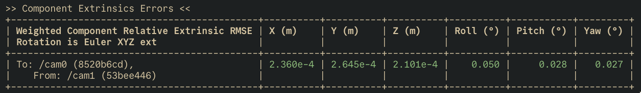
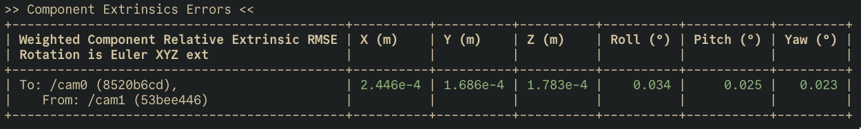
As you can see, the reprojection error is worse comparatively; however, the ray-alignment calibration holistically represents the 3D structure of the scene more faithfully. This improved 3D alignment can be seen by analyzing the relative extrinsics between the two cameras.
Minimizing Reprojection Error:
Minimizing Ray Error:
Putting it all together, we find our treatment of 3D information changes drastically between the two approaches.
Minimizing reprojection error induces large 3D ray error in regions where changes in real-world rays map to small changes in pixels
Minimizing over rays treats all 3D information fairly
Furthermore, we can directly compare ray alignment across cameras regardless of their field of view or pixel pitch; the same can’t be said for reprojection errors. This makes rays both better for evaluation and for faithfully modeling the geometry of a scene.
So why not start with Rays?
If the solution to Pinhole Obsession is to correctly model rays versus camera rays, then why do we not teach and implement this distinction from the beginning? The term Bundle Adjustment even comes from the idea of modifying geometric bundles of light rays to align with image coordinates. It seems very natural and intuitive to work with rays instead of camera rays in homogeneous coordinates. So why are real rays not commonly used in computer vision?
As it turns out, using real-world rays adds some complication to a computer vision processing pipeline. In our next post, we will cover the differential geometric foundations of rays and camera rays, cover a bit of Lie Theory, and show how to represent ray errors.


